1. Simulation Overview šÆ
Concept:Ā This app lets you plot a real-road route (distance) and the straight-line shortcut (displacement) between any two points on Earth.
Why it matters:Ā Students often treat distance and displacement as synonyms; visualising both on an actual map makes it crystal-clear thatĀ distance ā„ displacement and that only vectors carry direction. This tool can be accessed at https://prayogashaala.com/wp-admin/simulations/distance3.htmlĀ
2. How It Was Built š ļø
a. Construction Methods (Step-by-Step) šŖ
-
Prompt designĀ ā a detailed requirement list (see below) was fed to a generative-AI code assistant.
-
Skeleton generationĀ ā the model produced a single-page HTML file with Leaflet.js, CSS and vanilla JS.
-
Iterative refinementĀ ā successive prompts added GPS accuracy checks, map-click workflow, š input, a radius slider and a modal confirmation dialog.
-
TestingĀ ā routes were validated in Bangalore, Delhi and London to ensure the Haversine displacement matched Google Earth great-circle values.
-
User-configurable API keyĀ ā internal key hard-coding was replaced by a āš Geoapify API Keyā panel that stores the key inĀ
localStorage. A video showing how to obtain this API key step by step instructions is as shown below.
b. Prompt Used (Initial Seed) š¬
Create a complete web based physics simulation with the following specifications:
Core Functionality
Interactive map-based physics simulation demonstrating distance vs displacement concepts
ā¦the route animation must last 5 seconds, show a thick 10 px line, include car/bike/walk speeds, calculate efficiencyā¦
Technical Requirements
Leaflet.js only, Geoapify Places & Routing, responsive design, no external dependenciesā¦
Educational Features
Haversine displacement, route efficiency, misconceptions, student worksheetā¦
3. Software & Tools š»š§
4. Logic & Frameworks š§®
a. Underlying Logic š§āš¬
-
Distance (d):Ā sum of poly-line segment lengths returned by Geoapify route.
-
Displacement (Īr):Ā direct great-circle arc via the Haversine formula.
-
Efficiency:Ā Ī·= (Īr/d ) x 100ā%Ā
-
Travel time:Ā t=dvvehiclet=vvehicledĀ with preset speeds (š 50 km hā»Ā¹, š“ 20 km hā»Ā¹, š¶ 5 km hā»Ā¹).
A 5 sĀ setIntervalĀ loop interpolates 110 waypoints so the icon glides smoothly along the path while a 10 px āsnakeā line grows behind it.
5. Prompting Frameworks š§ āØ
6. How to Use the Simulation šš¹ļø
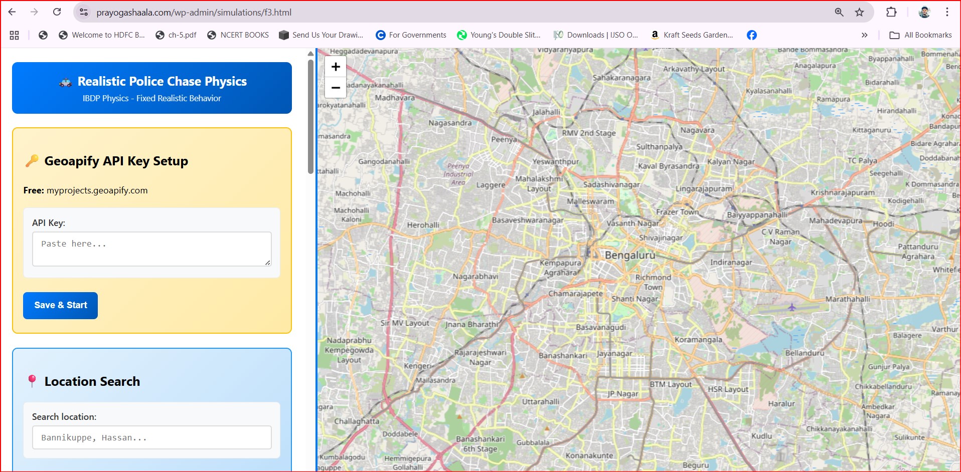
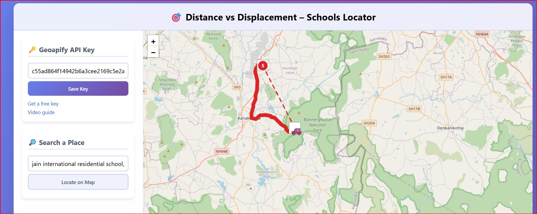
a. User Guide ( Click here to Open the Simulation )
Paste yourĀ Geoapify API keyĀ in the
panel āĀ Save.
Type a city or landmark āĀ Locate on Map.
ClickĀ
Click on MapĀ and tap the exact start point.
Adjust theĀ radius sliderĀ (0 ā 15 km).
HitĀ Find Nearby SchoolsĀ ā choose a school from the list.
Select aĀ vehicleĀ (
/
/
).
PressĀ
Start Animation. Watch the icon travel the route while results update in real time.
b. Tips & Tricks 
Drag the start marker to fine-tune its position before searching.
Set radius toĀ 0 kmĀ to test error handling when no POIs exist.
Compare efficiencies for walking vs driving in a dense city centre.
Worksheet Questions:
Why can efficiency exceed 90% in rural areas but fall below 30% downtown?
Design a looped route where displacement = 0 but distance > 0. What efficiency do you get?
Predict how efficiency changes if you double every poly-line waypoint.
7. What Makes It Unique š
a. Comparison with Other Simulations
Ā
b. Educational Value š
-
Misconception spotlight:Ā StudentsĀ seeĀ why āshortest pathā ā āshortest distanceā.
-
Authentic context:Ā Real roads anchor physics to everyday travel.
-
Prompt-engineering showcase:Ā Changing a single instruction reshapes both codeĀ andĀ pedagogy.
Whether youāre aĀ student,Ā educator, orĀ curious explorer, this simulation is your gateway to hands-on, AI-enhanced learning.Ā Dive in, experiment, and let the journey from physics to philosophy begin!Ā šš